AI, machine learning, and deep learning: Everything you need to know

There’s a lot of marketing buzz and technical spin on artificial intelligence, machine learning, and deep learning. Most of what’s out there is either too fluffy or too mathy, either too general or too focused on specific applications, too disconnected from business outcomes and metrics, and too undirected.

This article provides an overview of these related technologies by:

• Defining AI, machine learning, and deep learning, explaining the differences from traditional approaches, describing when to use them, and noting their advantages and disadvantages.
• Explaining how they complement business frameworks and enable business outcomes and metrics.
• Describing common types of machine learning and deep learning model training, algorithms, architectures, performance assessments, and obstacles to good performance.
• Providing examples of machine learning models and algorithms at work.
• Presenting a potential framework for AI implementation for business outcomes.

Why AI: AI in the business context

All organizations work to specific outcomes, and they juggle several business metrics and processes to achieve this, such as revenue, costs, time to market, process accuracy, and efficiency. Yet they have limited resources (money, time, people, and other assets). So, the problem boils down to making good decisions about resource allocation (what kind of resources, how many/much of them, what should they do, what capabilities do they need, etc.), and making those good decisions faster than competitors and faster than the market is changing.

Making these decisions is hard, but clearly, they become much, much easier when data, information, and knowledge are available. Assuming these inputs are available, they need to be aggregated and mined for nuggets. Analysts need time to pull tribal knowledge out of subject matter experts’ heads, to adjust to fluctuating business rules, to calibrate for personal biases where possible, and to spot patterns and to generate insights. Ideally, analysts and managers should (time permitting) assess multiple scenarios and run several experiments to increase confidence in their recommendations and decisions. Finally, the decisions need to be operationalized.

Enter AI, machine learning, and deep learning, which:

• Model the organization based on observations.
• Generate insights by simultaneously reviewing lots of factors and variables (far more than a person can achieve in a reasonable time period and cost constraint).
• Learn continuously as new observations are provided.
• Quantify the likelihood of outcomes (that is, predict what is likely to happen).
• Prescribe specific actions to optimize the business goals and metrics.
• Adjust rapidly to new business rules through faster retraining versus traditional slower reprogramming.

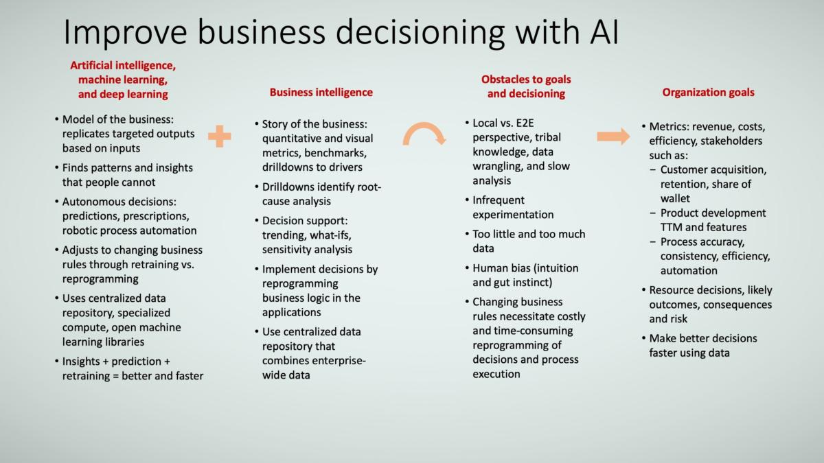
What makes AI, machine learning, and deep learning possible now is the proliferation of data volume and data types coupled with the lower costs of compute and storage hardware and tools. Web-scale companies (such as Facebook, Google, Amazon, and Netflix) have proven it works, and they are being followed by organizations in all industries. Combined with business intelligence, the trio of artificial intelligence, machine learning, and deep learning overcomes obstacles to decisioning, thereby facilitating organizations to achieve their business goals, as Figure 1 shows.

TRACE3

AI, machine learning, and deep learning apply to everyone in metrics-driven organizations and businesses.

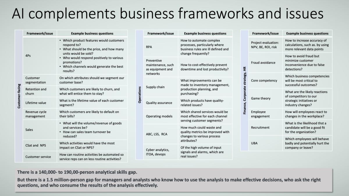
In its May 2011 publication “Big Data: The Next Frontier for Innovation, Competition, and Productivity,” McKinsey Global Institute stated that the gap for managers and analysts who know how to use the results of analytics stood at 1.5 million, an order of magnitude more than for those who produce the analytics (such as data analysts and data scientists).

Put another way, the chokepoint in the data value chain is not the data or the analytics; it’s the ability to consume the data/analytics in context and in an intelligent way for surgical action. This is an opportunity for business and process professionals to marry AI, machine learning, and deep learning to the business frameworks and concepts already understood so well. It’s a chance to define problems and hypotheses within those frameworks and concepts, and then to use AI, machine learning, and deep learning to find patterns (insights) and to test hypotheses that take too long to test, would otherwise be too expensive to identify and test, or are too difficult for people to carry out, as Figure 2 shows.

TRACE3

Organizations and businesses are increasingly turning to AI, machine learning, and deep learning because, quite simply, business is becoming more complex. There are too many things occurring at one time for us people to process; that is, there are too many data points (both relevant and not-so-relevant) for us to synthesize. Looked at it this way, too much data can be a liability (analysis paralysis, anyone?).

But AI, machine learning, and deep learning can turn that pile of data into an asset by systematically determining its importance, predicting outcomes, prescribing specific actions, and automating decision making. In short, AI, machine learning, and deep learning enable organizations and businesses to take on the factors driving business complexity, among them:

• Value chains and supply chains that are more global, intertwined, and focused on microsegments.
• Business rules that rapidly change to keep pace with competitors and customer needs and preferences.
• Correct forecasting and deployment of scarce resources to optimize competing projects/investments and business metrics.
• Need to simultaneously drive towards both increased quality and customer experience while reducing costs.

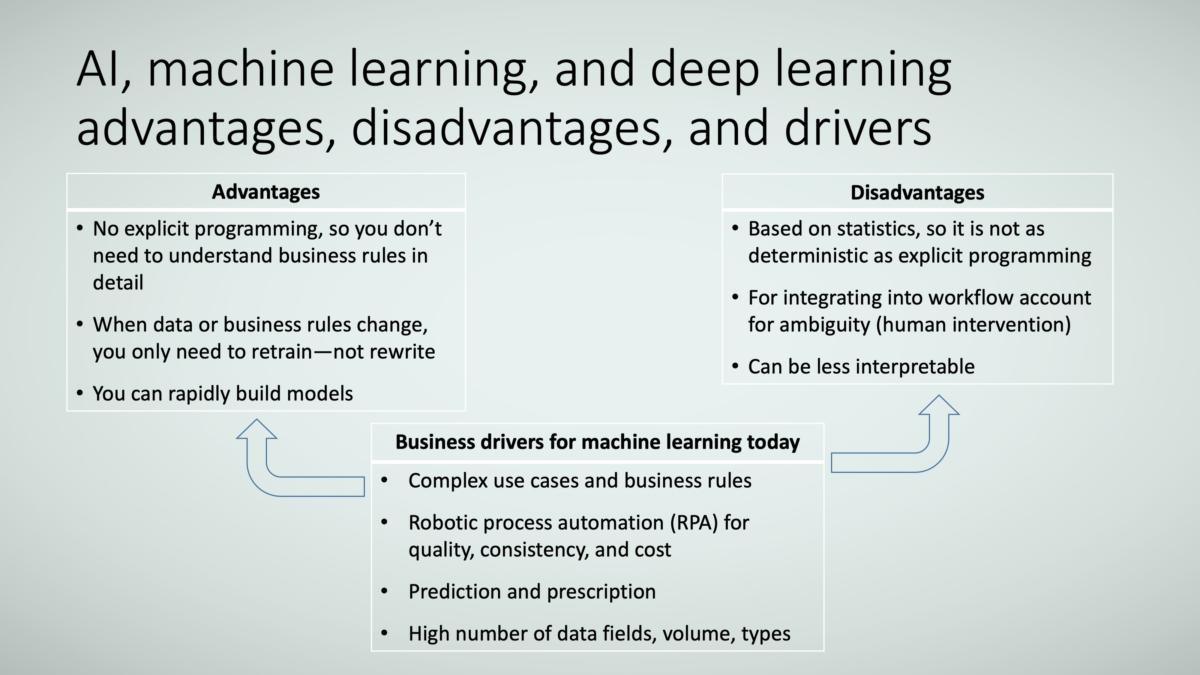
In many ways, AI, machine learning, and deep learning are superior to explicit programming and traditional statistical analysis:

• The business rules don’t really need to be known to achieve the targeted outcome—the machine just needs to be trained on example inputs and outputs.
• If the business rules change such that the same inputs no longer result in the same outputs, the machine just needs to be retrained—not reprogrammed—allecelerating response times and alleviating people of the need to learn new business rules.
• Compared to traditional statistical analysis, AI, machine learning, and deep learning models are relatively quick to build, so it’s possible to rapidly iterate through several models in a try-learn-retry approach.

However, AI, machine learning, and deep learning do have disadvantageous, as Figure 3 shows. Among them, they are still based on statistics, so there is an element of uncertainty in the output. This makes the integration of AI, machine learning, and deep learning into the workflow tricky because high ambiguity in the machine’s decisions should likely be handled by a person. And to improve the machine’s accuracy, mistakes (and right answers) should be fed back to the machine to be used for additional training (learning).

Additionally, AI, machine learning, and deep learning models can be less interpretable; that is, it may not be clear how they arrive at their decisions. This is particularly true of complex deep learning models with many “layers” and “neurons”; such lack of clarity may be of particular concern in highly regulated industries. It should be noted that there is a lot of research focused in this area, so perhaps it won’t be a disadvantage in the future.

TRACE3

Given the advantages and disadvantages, when might it be appropriate to use AI, machine learning, and deep learning? Here are some ideas:

• The juice is worth the squeeze: There’s a high-potential business outcome but traditional approaches are too cumbersome, time-consuming, or just not appropriate.
• Relevant data is available and accessible.
• Subject matter experts believe the data contain meaningful signal (that is, insight can be gleaned from the data).
• The problem definition ties to a machine learning or deep learning problem, such as classification, clustering, or anomaly detection.
• The success of use cases can be mapped to machine learning and deep learning model performance metrics, such as precision-recall and accuracy.

AI defined: The natural progression from BI to AI

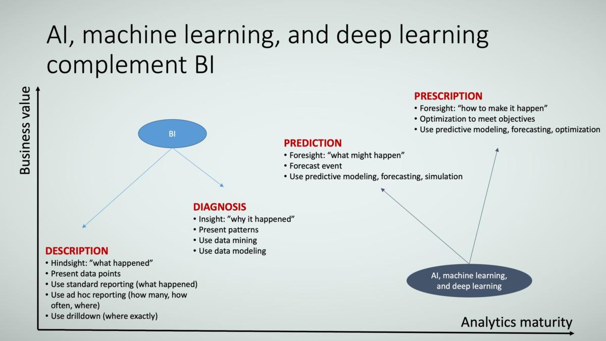
AI, machine learning, and deep learning are a natural progression of business intelligence. Where BI describes and diagnoses past events, AI, machine learning, and deep learning try to predict the likelihood of future events and prescribe how to increase the likelihood of those events actually occurring. A simple example illustrating this is the GPS guiding you from point A to point B:

• Description: What route did the vehicle take, and how long did it take?
• Diagnosis: Why did the vehicle take a long time at a particular traffic light (assuming the GPS platform/tool tracks things like accidents and vehicle volume)?
• Prediction: If a vehicle is going from point A to point B, what is the expected ETA?
• Prescription: If a vehicle is going from point A to point B, what route should the vehicle take to achieve the expected ETA?

Prediction in AI

One example of prediction is sentiment analysis (the probability of someone liking something). Let’s assume you can track and store the textual content of any user posting (such as tweets, updates, blog articles, and forum messages). You can then build a model that predicts the user’s sentiment from his or her postings.

Another example is increasing customer conversion: people are more likely to sign up for subscriptions if they’re offered a chance to win a prize they want—so you can predict which prizes will lead to the highest number of conversions.

Prescription in AI

Prescription is about optimizing business metrics in various processes, such as marketing, sales, and customer service, and it’s accomplished by telling the prescriptive analytics system what metrics should be optimized. This is like telling the GPS what you want to optimize, such as least fuel consumption, fastest time, lowest mileage, or passing by the largest number of fast-food joints in case you get a craving for something. In a business setting, you might target increased conversion by 10 percent, sales by 20 percent, or net promoter score (NPS) by five points.

From there, the prescriptive analytics system would prescribe a sequence of actions that leads to the corresponding business outcomes you want.

Say you want to achieve a 10-percent conversion lift. The system may prescribe:

• Reducing the frequency of your direct mail marketing by 15 percent, while
• simultaneously increasing your Twitter and Facebook engagements by 10 and 15 percent, respectively, then
• when your aggregate social media engagement reaches 12 percent, start directing the public to your customer community portal for customer-to-customer engagement.

These prescriptive actions are like the turns that your GPS system advises you to take during the journey to optimize the goal you set.

The relationship among BI, statistics, and AI

Here’s one way to define the difference among BI, statistics, and AI:

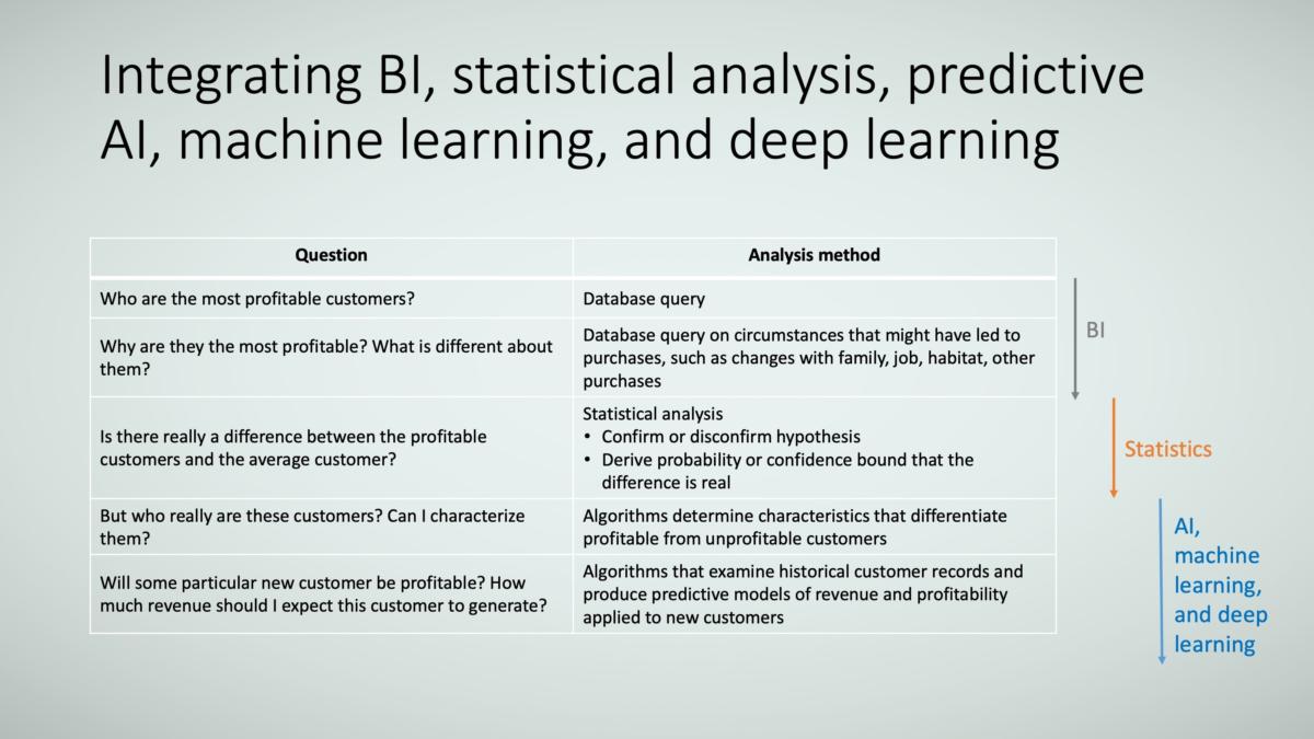
• BI is traditionally query-oriented and relies on the analyst to identify the patterns (such as who are the most profitable customers, why are they the most profitable, and what attributes that set them apart, such as age or job type).
• Statistics also relies on the analyst to understand the properties (or structure) of the data to find information about the population in the data, but it adds mathematical rigor in extrapolating to generalization (such as if there is a difference between these customer segments in real life versus what is found in the sample data).
• AI, machine learning, and deep learning rely on algorithms (not analysts) to autonomously find patterns in the data and enable prediction and prescription.

TRACE3

Please note that BI, statics, and AI, machine learning, and deep learning can do more than what is described in Figure 5; this example simply demonstrates how these methods can answer a series of progressive business questions.

TRACE3

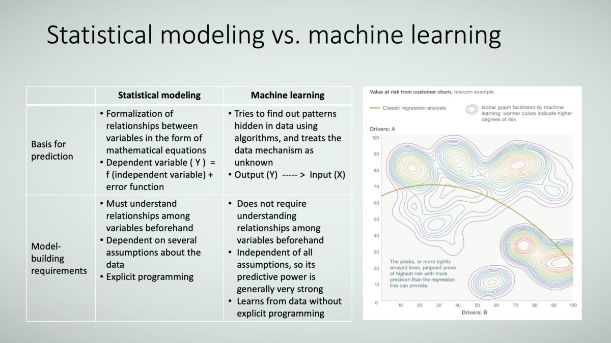
While statistical modeling on one side and machine learning and deep learning on the other are both used to build models of the business situation, there are some key differences between the two, as Figure 6 shows. In particular:

• Statistical modeling requires a formal mathematical equation between the inputs and outputs. In contrast, machine learning and deep learning don’t try to find that mathematical equation; instead they simply try to re-create the output given the inputs.
• Statistical modeling requires an understanding between the variables and makes assumptions about the statistical properties of the data population. Machine learning and deep learning do not.

TRACE3

Typically, because statistical modeling requires a mathematical equation and an understanding of the relationships among the data, statistical models take a relatively long time to build as the statistician studies and works with the data. But if completed successfully—that is, the equation is found and the statistical relationships among the data are very well understood—the model can be killer.

Machine learning and deep learning models, on the other hand, are very fast to build but may not achieve high performance to start. But because they are so easy to construct in the early stages, many algorithms can be tried simultaneously with the most promising of them continuously iterated until model performance becomes extremely good.

Machine learning and deep learning models also have the added advantage of continuously learning from new data “on their own,” and thus improving their performance.

Should the nature of the data change, the machine learning and deep learning models simply need to be retrained on the new data; whereas the statistical models typically need to be rebuilt in whole or in part.

Machine learning and deep learning models also excel in solving highly nonlinear problems (it’s just harder for people to do this—those equations get very long!). This attribute of machine learning and deep learning really comes in handy as microsegments become the norm (think customer segments of one, mass customization, personalized customer experience, and personal and precision medicine), and processes and root-cause analysis becomes increasingly multifactored and interdependent.

How AI, machine learning, and deep learning differ

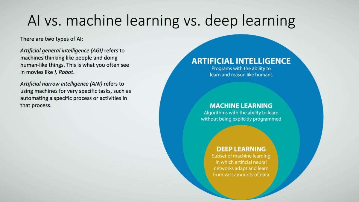
So far, I have lumped together AI, machine learning, and deep learning together. But they are not exactly the same, as Figure 7 shows.

TRACE3

Generally speaking:

AI is where machines perform tasks that are characteristic of human intelligence. It includes things like planning, understanding language, recognizing objects and sounds, learning, and problem solving. This can be in the form of artificial general intelligence (AGI)or artificial narrow intelligence (ANI).

• AGI has all the characteristics of human intelligence, with all our senses (maybe even more) and all our reasoning, and so can think just like we do. Some describe this as “cognitive”—think C3PO and the like.
• ANI has some facets of human intelligence but not all; it’s used to perform specific tasks. Examples include image classification in a service like Pinterest and face recognition on Facebook. ANI is the current focus of most business applications.

Machine learning is where machines use algorithms to learn and execute tasks without being explicitly programmed (that is, they do not have to be provided specific business rules to learn from the data; put another way, they don’t need instructions such as “if you see X, do Y”).

Deep learning is a subset of machine learning, generally using artificial neural networks. The benefit of deep learning is that in theory it does not need to be told what data elements (or “features” in machine learnig speak) are important, but most of the time, it needs large amounts of data.

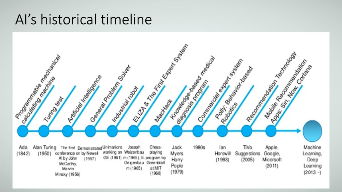
Figure 8 shows the timeline of AI’s evolution.

TRACE3

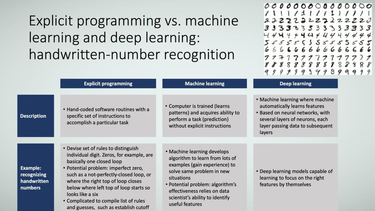
The differences among explicit programming, machine learning, and deep learning can be better understood through the example of handwritten number recognition. To a person older than five years old, recognizing handwritten numbers isn’t hard. We’ve learned (been trained) over the years by parents, teachers, siblings, and classmates.

Now imagine getting a machine to do the same through explicit programming. In explicit programming, you have to tell the machine what to look for. For example, a round object is a zero, a line that goes up and down is a one, and so on. But what happens if the object isn’t perfectly round, or the ends don’t touch so it’s not fully round? What happens when the line doesn’t go up and down but instead tips sideways, or if the top part of the line has a hook (like “1”)—is it now closer to 7? The many variations of handwritten letters make it difficult to write an explicit program; you would be consistently adding new “business rules” to account for the variations.

As Figure 9 shows, in the machine learning approach, you would show the machine examples of 1s, 2s, etc., and tell it what “features” (important characteristics) to look for. This feature engineering is important because not all characteristics are important. Examples of important characteristics might be number of closed loops, number of lines, direction of lines, number of line intersections, and positions of intersections. Examples of unimportant characteristics might be color, length, width, and depth. Assuming you feed the machine the right features and provide it with examples and answers, the machine would eventually learn on its own how important the features are for the different numbers, and then hopefully be able to distinguish (or classify) the numbers correctly.

Notice that with machine learning you have to tell the machine the important features (that is, what to look for), so the machine is only as good as the person identifying the appropriate features.

The promise of deep learning is that no one has to tell the machine what features to use (that is, which ones are most important)—it will automatically figure this out. All you need to do is to feed it all the features from which it will select the important features on its own. While this an obvious advantage, it comes at a price in the form of high-data-volume requirement and long training time that requires significant computational processing capabilities.

TRACE3

AI model concepts: an overview

The idea behind machine learning and deep learning models is they learn from data they are given (things they have seen before), and then can generalize to make good decisions on new data (things they have not seen before).

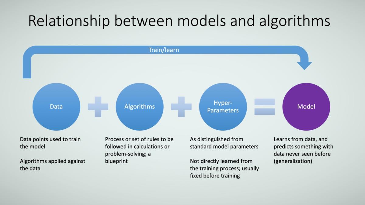
But what constitutes a model? One definition of models is that they consist of three components:

• Data: Historical data is used to train the model. For example, when learning to play the piano, the data you are fed is different notes, different types of music, different composer styles, etc.
• Algorithms: General rules that models use for the learning process. In the piano example, your internal algorithm might tell you to look for the musical notes, how to move your hands on the keys, how and when to press the pedals, etc. Figure 10 shows the relationship between models and algorithms.
• Hyperparameters: These are “knobs” that data scientists adjust to improve the model performance, and they are not learned from the data. Again using the piano example, hyperparameters include how often you practice the musical piece, where you practice, time of day you practice, piano you use for practice, etc. The thinking is that adjusting these “knobs” improves your ability to learn how to play the piano.

When you put all of this together, you become a piano-playing model. In theory, depending on how well you’re trained, new musical pieces you’ve never seen before could be placed in front of you and you’d be able to play them.

TRACE3

Types of machine learning

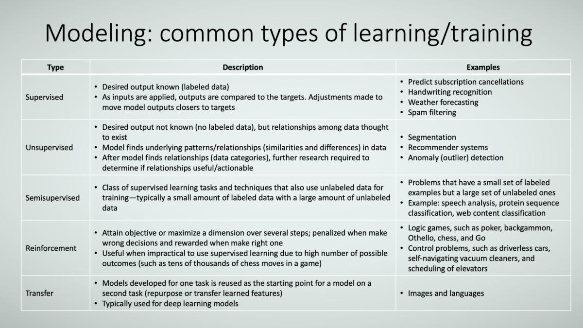
Machines, just like people, can learn in different ways, as Figure 11 shows. I’ll again use the piano-training analogy to explain:

• Supervised: Your instructor shows or tells you both the right way and the wrong way to play. In an ideal situation, you are given equal numbers of examples of how to play the right and wrong ways. Essentially, the training data consists of a target/outcome variable (or dependent variable) that is to be predicted from a set of predictors (independent variables). Using these sets of variables, you generate a function that maps inputs to desired outputs. The training process continues until the model achieves a desired level of performance on the training data. A business example of supervised training is showing the system examples of loan applications (consisting of predictors like credit history, work history, asset ownership, income, and education) that were approved or rejected (the target outcomes and decisions).
• Unsupervised: You’re on your own—nobody tells how you to play, so you make up your own ideas of right and wrong, with the goal of optimizing a parameter that’s important to you, such as speed of finishing the piece, the ratio of loud notes to soft notes, or number of unique keys you touch. Essentially, data points have no labels associated with them to inform you right or wrong. Instead, the goal is to organize the data in some way or to describe its structure. This can mean grouping it into clusters or finding different ways of looking at complex data so that it appears simpler or more organized. Unsupervised learning is usually less effective at training the model than supervised learning, but it may be necessary when no labels exist (in other words, the “right” answers are not known). A common business example is market segmentation: It’s frequently unclear what the “right” maret segments are, but every marketer is looking for segments of natural affinities so they can approach those segments with just the right message, prootions, and products.
• Semisupervised: A combination of supervised and unsupervised. This is used where there is not enough supervised data. In the piano example, you would receive some instruction but not a lot (maybe because lessons are expensive or there aren’t enough teachers).
• Reinforcement: You’re not told what the right and wrong way to play is, and you don’t know what parameter you’re trying to optimize, but you are told when you do something right or wrong. In the case of piano training, your teacher might hit your knuckles with a ruler when you play the wrong note or play with the wrong tempo, and she gives you a backrub when you play things well. Reinforcement learning is very popular right now because, in several situations, there isn’t enough supervised data available for every scenario, but the “right” answer is known. For example, in the game of chess, there are too many permutations of moves to document (label). But reinforcement learning still lets tells the machine when it makes right and wrong decisions that advance to ward winning (such as capturing pieces and strengthening positions in chess).
• Transfer learning: You use your knowledge of playing the piano to learn another instrument because you’ve built certain transferable skills (such as the ability to read notes and maybe even developing nimbleness in your hands) that you can build on to learn how to play the trumpet. Transfer learning is used because it reduces learning time, which can be significant (several hours or even several days) for models that use deep learning architectures.

TRACE3

Common machine learning algorithms

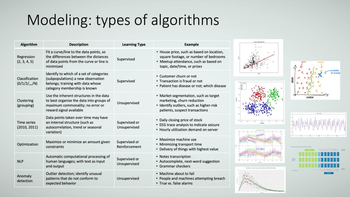
As Figure 12 shows, common algorithm types include:

• Regression is simply drawing a curve or line through data points.
• Classification is determining to what group something belongs. Binary classification (two groups) is determining if something belongs to a class or not, such as whether the animal in the picture is a dog or not. Sticking with the animal example, multiclass classification (more than two groups) is whether the animal is a dog, cat, bird, etc.
• Clustering is similar to classification, but you don’t know the classifications ahead of time. Again using the examples of animal pictures, you may determine that there are three types of animals, but you don’t know what those animals are, so you just divide them into groups. Generally speaking, clustering is used when there is insufficient supervised data or when you want to find natural groupings in the data without being constrained to specific groups, such as dogs, cats, or birds.
• Time series assumes that the sequence of data is important (that the data points taken over time have an internal structure that should be accounted for). For example, sales data could be considered time-series because you may want to trend revenue over time to detect seasonality and to correlate it with promotion events. On the other hand, the order of your animal pictures doesn’t matter for classification purposes.
• Optimization is a method of achieving the best value for multiple variables when they do not move in the same direction.
• NLP (natural language processing) is the general category of algorithms that try to mimic human use and understanding of languages, such as chatbots, scrubbing unstructured writing like doctor’s notes for key data fields, and autonomous writing of news articles.
• Anomaly detection is used to find outliers in the data. It is similar to control charts but uses lots more variables as inputs. Anomaly detection is especially useful when “normal” operating parameters are difficult to define and change over time, and you want your detection of abnormalities to adjust automatically.

TRACE3

Deep learning models

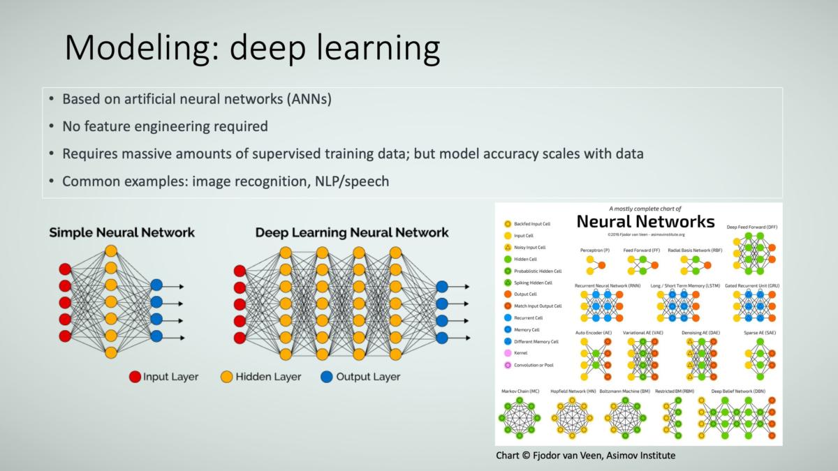
Deep learning is based on the concept of artificial neural networks (ANNs). In that way, they work like human brains where synapses become stronger or weaker based on feedback of some sort, and neurons fire based on specified conditions. Hard problems are being solved through deep learning models, including self-driving cars, image detection, video analysis, and language processing. Figure 13 shows their key characteristics.

Lest you think that deep learning models are the only things that should be used, there are some caveats:

• First, they require large amounts of data—generally much more than machine learning models. Without large amounts of data, deep learning usually does not perform as well.
• Second, because deep learning models require large amounts of data, the training process takes a long time and requires a lot of computational processing power. This is being addressed by ever more powerful and faster CPUs and memory as well as newer GPUs and FPGAs (field-programmable logic arrays).
• Third, deep learning models are usually less interpretable than machine learning models. Interpretability is a major area of deep learning research, so perhaps this will improve.

TRACE3

How to measure machine learning model performance

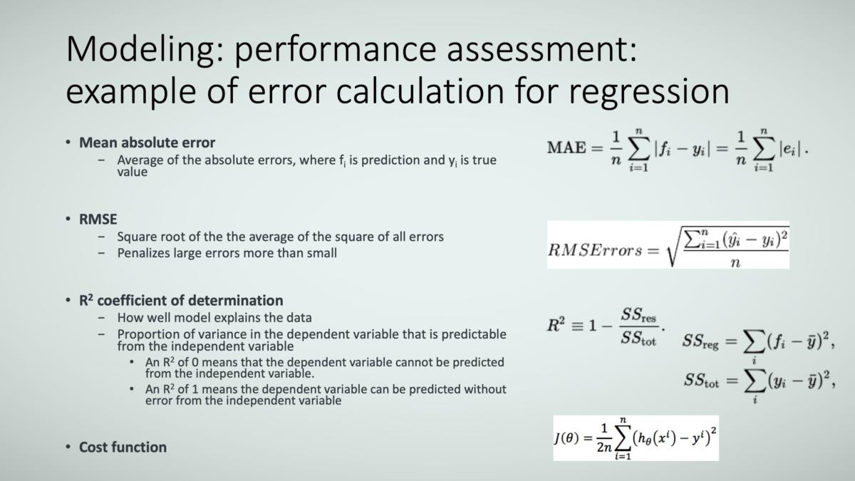
Models, just like people, have their performance assessed. Here are a few ways to measure the performance of a relatively simple regression model. The MAE, RMSE, and R² performance metrics are fairly straightforward, as Figure 14 shows.

All these can be considered a type of cost function, which helps the model know if it’s getting closer or farther away from the “right” answer, and if it’s gotten “close enough” to that answer. The cost function tells the model how far it has to go before it can take new data it hasn’t seen before and output the right prediction with a high enough probability. When training the model, the goal is to minimize the cost function.

TRACE3

Precision versus recall in classification models

Once the cost function has done its job of helping the model head in the direction of the “right answer” based on training data (data it is being shown), you need to evaluate how well the model performs on data it hasn’t yet seen. Let me explain this in the context of classification models (models that determine whether something is in one group or another, such as if the picture is a dog, cat, rat, etc.).

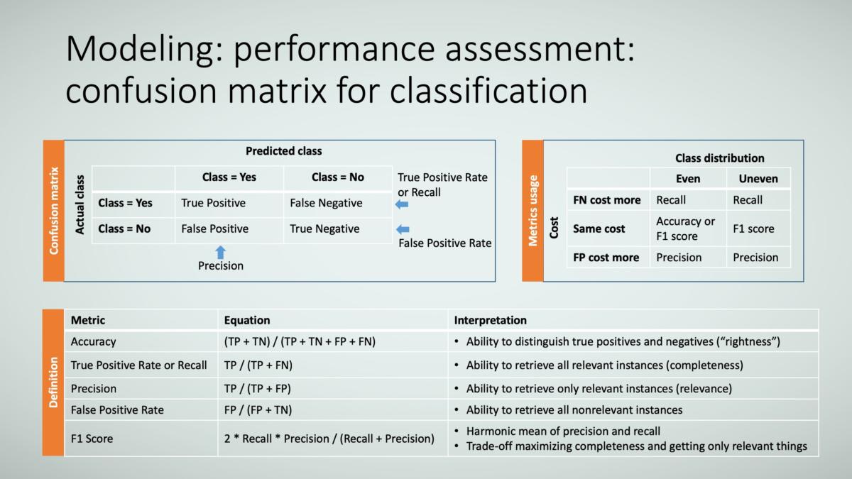
To assess the performance of classification models (see Figure 15), you use the equation for accuracy (as detailed below). However, it’s generally accepted that when the training data exhibits class imbalance, the accuracy metric might be misleading, so you use metrics called precision and recall instead. Here’s what these terms mean:

• Class imbalance: The data is skewed in one direction versus other directions. Consider the example of predicting whether a credit card transaction is fraudulent. The vast majority of transactions are not fraudulent, and the data set will be skewed in that direction. So, if you predicted that a given transaction is not fraud, you’d probably be right—even if you know nothing about transaction itself. Applying the accuracy metric in this example would mislead you to think you’re doing a great job of predicting transactions that are not fraudulent.
• Precision is a measure of relevance. Pretend you use your search engine to find the origin of the tennis score “love.” Precision measures how many of the items returned are really about this versus links to how much people love tennis, how people fell in love playing tennis, etc.
• Recall is a measure of completeness. Using the same example of the tennis score “love,” recall measures how well the search engine captured all the references that are available to it. Missing zero references is amazing, missing one or two isn’t too bad, missing thousands would be terrible.

Unfortunately, in the real world, precision and recall are traded off; that is, when one metric improves, the other metric deteriorates. So, you’ve got to determine which metric is more important to you.

TRACE3

Consider the example of a dating app that matches you with compatible people. If you’re great-looking, rich, and have a sparkling personality, you might lean towards higher precision because you know there will be a lot of potential matches, but you only want the ones that are a real fit, and the cost for you to screen potential matches is high (hey, you’re busy building an empire—you’ve got millions of things to do). On the other hand, if you’ve been looking for someone for a long time and your mother’s been on your back, you might lean toward recall to get as many potential matches as possible. The cost of sorting through potential suiters is relatively low compared to the constant nagging from your mother! To assess how well the model balances precision and recall, the F1 score is used.

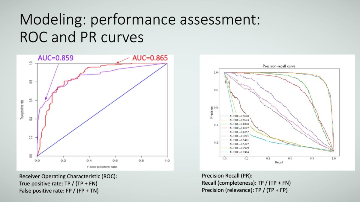
These metrics can be plotted on a graph, as Figure 16 shows; one is called the ROC curve (receiver operating characteristic curve) and the other is the PR curve (precision-recall curve). A perfect curve (which you will never get unless you cheat!) is a curve that goes up the Y axis to 1 and then goes across the top. In the case of the ROC curve, a straight line across the diagonal is bad—this means that model predicts true positives and true negatives equally at 50 percent rates (no better than random guesses). These metrics are frequently converted to an area under the curve (AUC), so you’ll see terms like AUC ROC and AUC PR.

TRACE3

Why building machine learning models can be hard

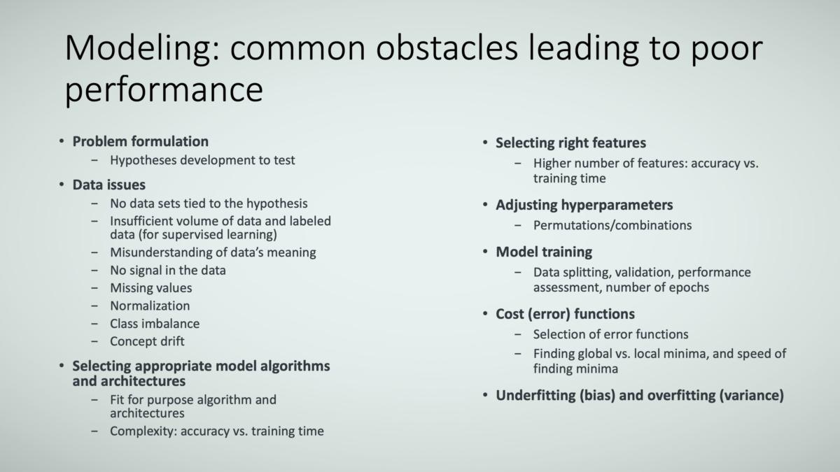
Now that you understand what a model is and how to judge a model’s performance, let’s explore why building a well-performing model can be hard. There are several reasons, as Figure 17 shows. Among them: problem formulation, data issues, selecting the appropriate model algorithm and architectures, selecting the right features, adjusting hyperparameters, training models, cost (error) functions, and underfitting (bias) and overfitting (variance).

Be aware that data science, just like any other science, is both an art and science. Of course, there are always brute-force ways to do things, but those approaches can be time-consuming, may miss insights, and may just plain get things wrong. The current approach of data science is to pool the knowledge of subject matter experts (such as lines of business, operations, and transformation and improvement specialists) and data scientists to create models that fulfil the business needs.

TRACE3

Overfitting versus underfitting

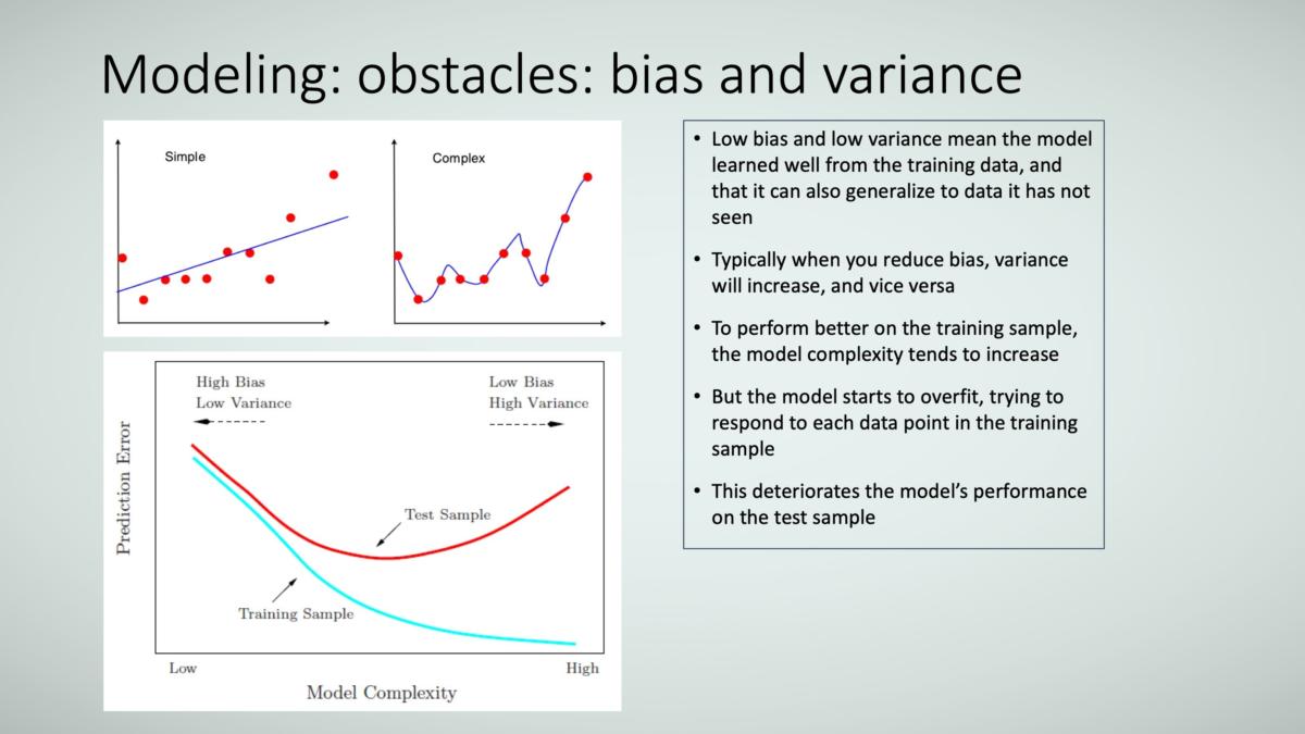
Overfitting and underfitting are particularly popular problem outcomes, so let’s delve into them a bit. As Figure 18 shows, they involve bias and variance.

Overfitting (high variance) means that the model responds too much to variations in the data, such that it hasn’t really learned the true meaning and instead “memorized” the data. It would be the same as you reading a math book in school and, when given a test on it, know the answers only to the three examples given in the book. When the teacher asks you these math problems (say, 2+1=3, 7+2=9, and 4+2=6), you get them right. But when she asks you something different—say, 1+1=?—you don’t know the answer. That’s because you haven’t learned what addition is, even though you know the answers to the examples. (By the way, don’t tell my professors, but this method saved my bacon in college back in the day!)

Underfitting (high bias) is the opposite problem in that you refuse to learn something new. Maybe you know how to do addition in base 10. But now circumstances have changed, and you’re asked to do addition in base 16. If you exhibit high bias, you’ll continue to do base-10 addition and not learn base-16 addition, and so you get the wrong answers.

Both are problems, and data science has mechanisms to help mitigate them.

TRACE3

Machine learning model examples

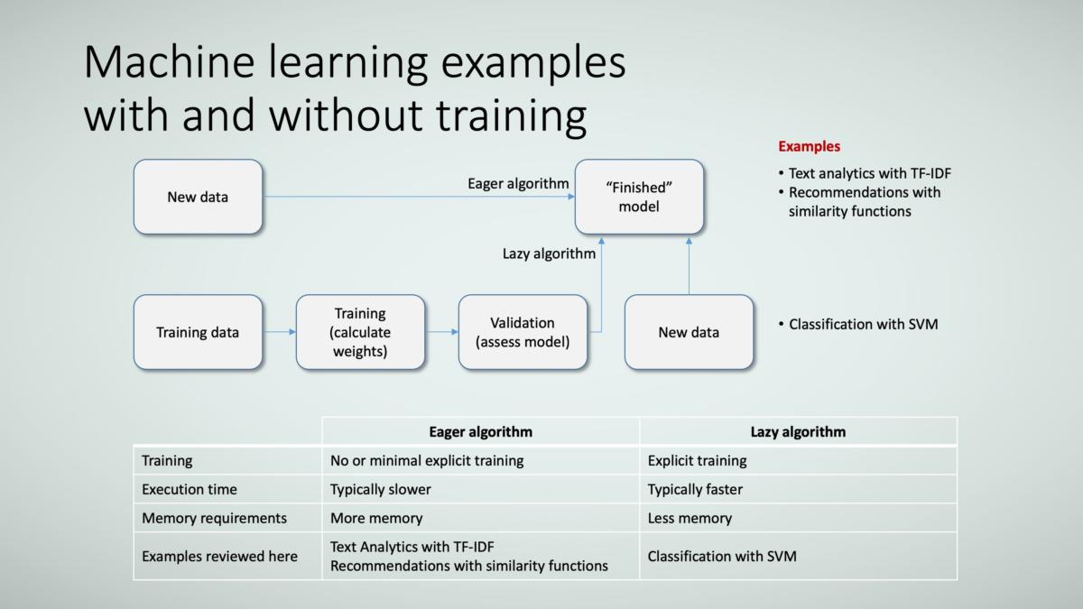
Let’s go through a couple of machine learning examples of using two types of algorithms: eager algorithms and lazy algorithms. Figure 19 shows examples of both.

Eager algorithms don’t use explicit training (the first path in the diagram), whereas lazy algorithms are explicitly trained (the second path in the diagram). Because eager algorithms aren’t explicitly trained, their training phase is fast (nonexistent, actually), but their execution (or inference phase) is slower than the trained lazy algorithms. Eager algorithms also use more memory because the entire data set needs to be stored, while the data used to train the lazy algorithm can be discarded once training is completed, using less overall memory.

TRACE3

Example: Document search using TF-IDF

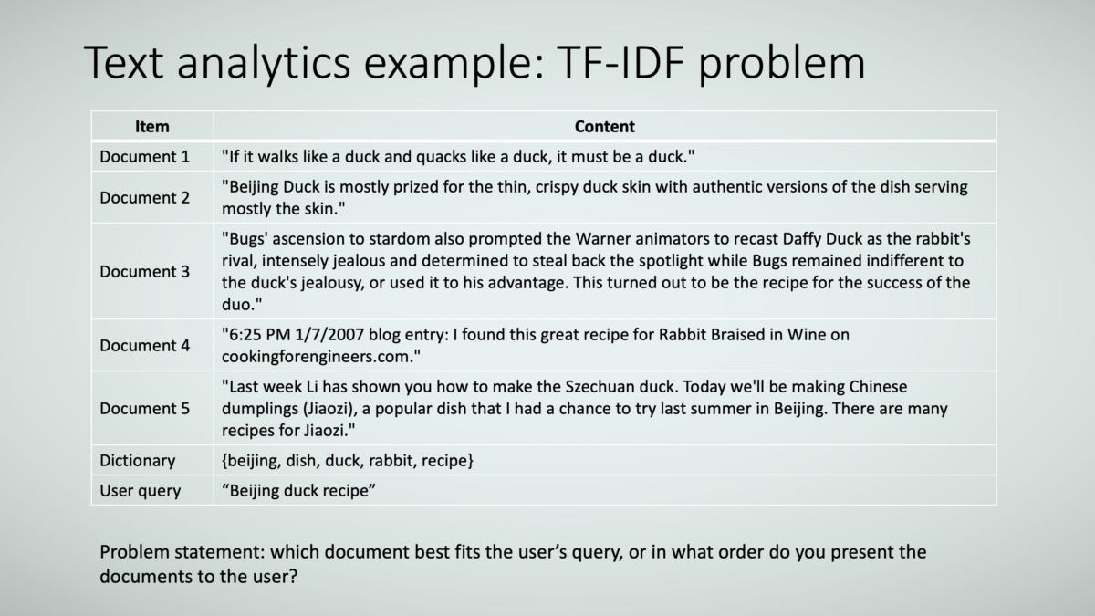
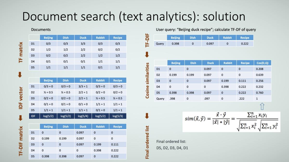
In this first example of an eager algorithm applied to text analytics, I’m using an algorithm called TF-IDF. I’ll explain what TF and IDF mean shortly, but let’s first be clear on the goal of this example. There are five simple, short documents (Documents 1 to 5), as Figure 20 shows. There’s also a dictionary of keywords for these documents; the dictionary is used for keyword searches. And there is also a user who has a query. The goal is to retrieve documents that best fit the user’s query. In this example, you want to return the five documents in order of prioritized relevance.

TRACE3

First, let me explain clarify the TF and IDF acronyms. TF stands for term frequency, or how often a term appears (that is, the density of that term in the document). The reason you care is because you assume that when an “important” terms appear more frequently, the document it’s in is more relevant; TF helps you map terms in the user’s query to the most relevant documents.

IDF stands for inverse document frequency. This is almost the opposite thinking—terms that appear very frequently across all documents have less importance, so you want to reduce the importance weight of those terms. Obvious words are “a,” “an,” and “the,” but there will be many others for specific subjects or domains. You can think of these common terms as noise that confuses the search process.

Once TF and IDF values are calculated for the documents and the query, you just calculate the similarity between the user’s query and each document. The higher the similarity score, the more relevant the document. Then you present those documents to the user in order of relevance. Easy right?

Now that you understand how it’s done, you just have to do the calculations. Figure 21 shows the solution.

TRACE3

Let’s walk through the calculations. By the way, you’ll see there are several matrices. Machine learning and deep learning models do a lot of their calculations using matrix math. You’ll want to be aware of that as you work with data scientists; you’ll want to help them get the data into these types of formats in a way that makes sense for the business problem. It’s not hard, but it’s part of the art of the data science preprocessing stage.

In the first TF matrix, you calculate the normalized (“relative”) frequency of each keyword (as specified in the dictionary) for each document. The numerator represents the word count frequency in that document, and the denominator represents the maximum number of times that word appeared in any give document; in other words, it’s the maximum value across all the numerators.

In the second matrix, you add an IDF vector in the last row for each term in the dictionary. You just apply the equation you’ve been given: IDF(t) = log(N/n(t)), where

• N = number of recommendable documents
• n (t) = number of documents in which keyword t appears

The next step is to create the TF-IDF matrix for the documents by multiplying each row of the documents by the last IDF row. Now you’re done with the document matrix. Repeat the same process to create the user-query matrix.

Finally, combine the two matrices and calculate the similarity between each document and the user query. In this case, you use an equation to calculate similarity called cosine similarity (there are other similarity calculations you can use as well). The equation is represented in the figure, and the values are in the last column. Notice that the similarity value between the user query and itself is 1—as it should be because it’s being compared to itself.

From here, you can sort the similarity values (in the last column of the matrix) from highest to lowest, thus presenting the user with documents from most to least relevant. Now you’re done! Notice there was no “training” of the model; you just applied a few equations.

Example: Pet recommendations using collaborative and content-based approaches

Let’s go through another example of an eager machine learning algorithm used in a recommender engine, similar to what you might see from many websites. In this case, you have data on four pet lovers, and you know their preference in terms of the type of pets they like and how much they like specific pets. Let’s assume there is a fifth pet lover (Amy) about whose preference you know less.

Your goals are two-fold: Predict the rating that Amy would give to a specific pet, and predict the preference of pets that Amy may like if you know her preferences of pet attributes. You should see that this closely resembles a similarity problem, using similarity of attributes between people you know more about to someone you know less about.

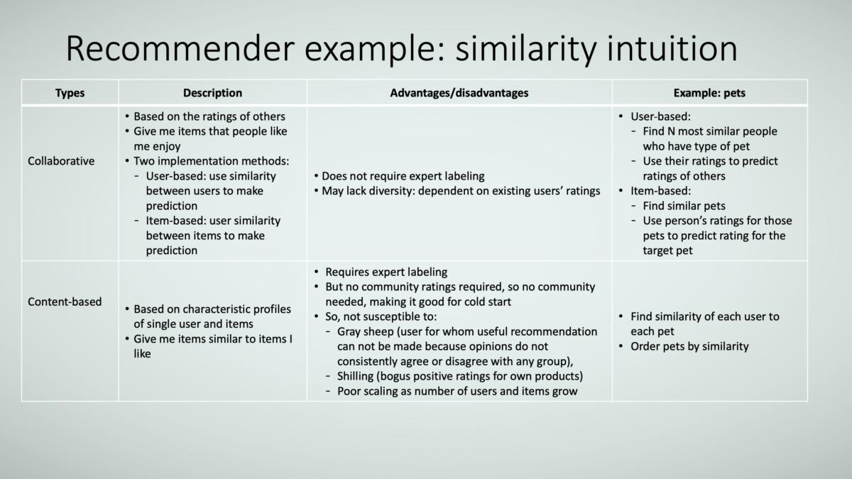
There are two ways to determine similarity in recommendation systems: collaborative and content-based, and collaborative can be further defined as user-based or item-based.

In the collaborative method, you need the ratings of users in the community. Applying this through the user-based approach, you predict what users like based on the likes of similar users in the community. By contrast, using the item-based approach, you predict what users like based on similarity among items that the community likes.

The content-based method does not use ratings of users in the community. Instead, it’s based on the characteristics of the items themselves, and the value (or label) assigned to these characteristics are provided by a domain expert.

Each method has its advantages and disadvantages, as Figure 22 shows.

TRACE3

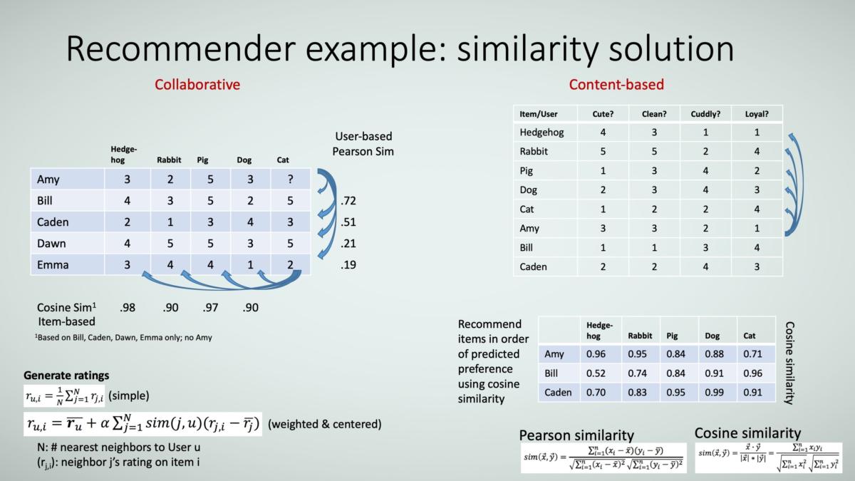
Consider this example: In the collaborative method, you use the pet ratings of other users to predict an individual’s unknown rating of a pet.

First, try the user-based approach. Because you are comparing aggregate individual’s ratings that can be skewed by human bias (that is, their baselines can be varied), you use a similarity function called the Pearson similarity (see the equation in the figure) that tries to correct for user bias by normalizing the ratings (that is, by subtracting the average of the ratings from each user rating). Working through the example, you see that Alice’s ratings are most similar to Bill’s ratings, so you can assume Amy’s missing rating would be the same as Bill’s.

Now try the item-based approach. In this approach, you don’t focus on individuals’ ratings but instead on the items’ ratings. And because the items’ ratings are a composite of ratings provided by several individuals, you don’t have to be as concerned about bias, so you can use the cosine similarity function (see the equation in the figure). Here, you see that Cat is most similar to Hedgehog, so you can infer that Amy’s rating for Cat would be the same as her rating for Hedgehog.

Finally, try the content-based approach. This approach doesn’t require the ratings of community members. Instead, an expert has labeled the data—in this case, the attributes (cute, clean, cuddly, loyal) of each pet type. If you know an individual’s preference for each attribute, you can use the cosine similarity function to predict the pets that the individual is most likely to enjoy. In this example, Amy is most likely to enjoy, in order of descending preference, Hedgehog, Rabbit, Dog, Pig, then Cat.

Let’s get into the math a bit. As an example, to determine Amy’s score for Hedgehog, you find the similarity between Hedgehog’s pet attributes and Amy’s ratings of importance of pet attribute:

• The Hedgehog’s vector is (4,3,1,1)
• Amy’s vector is (3,3,2,1)
• You need to find similarity between these two vectors
• Cosine similarity = [4(3) + (3)(3) + (1)(2) + (1)(1)] / [SQRT(4^2 + 3^2 + 1^2 + 1^2) * SQRT(3^2 + 3^2 + 2^2 + 1^2)] = .96

For the collaborative method, you use Pearson equation because it normalizes ratings across users (who can be inconsistent in their ratings). If you have objective ratings (such as ratings not based on people with different scales), you can use cosine similarity. Figure 23 shows the solution.

Here are the variables in the equations:

• u: user
• i: item to be rated
• N: # nearest neighbors
• j: neighbor
• r_j,I: j’s rating on i
• r_j bar: average of j’s ratings
• r_u bar: average of user’s rating
• alpha: scaling factor for ratings; 1 means use as is (there is no right value for alpha; it’s one of those hyperparameters) described earlier that an experienced data scientist can adjust to derive better results given the problem objective and context)

TRACE3

Example: Lazy algorithm using support vector machine (SVM)

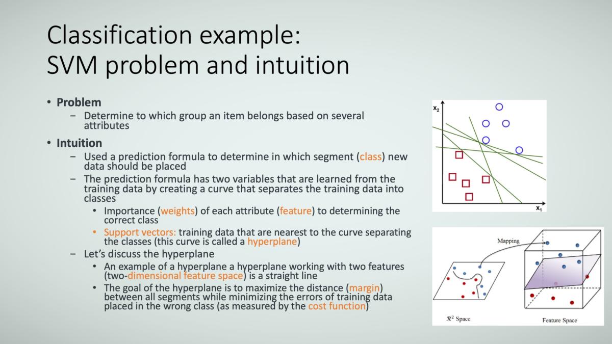
Finally, here’s an example of a lazy machine learning algorithm called the support vector machine (SVM). In this approach, you want to determine which group an item belongs, such as whether a new customer ends up being a highly or lowly profitable customer. To accomplish this using SVM, you need to calculate two parameters:

• Weights (importance) of each attribute (examples of attributes might be the customer’s income, number of family members, profession, and educational achievement)
• Support vectors, which are the data sets that are nearest to the curve (called a hyperplane) that separates the groups.

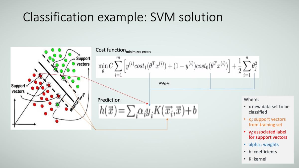
You then take these two parameters and plug them into an equation, as Figure 24 shows.

The way you calculate these parameters is to use the available data sets, and this is what is referred to as training the data.

TRACE3

Figure 25 shows the equation used to make the prediction under the Prediction label. Values that are calculated during the training phase are:

• The weights (the alphas and thetas) used to minimize the cost function.
• The support vectors x_i, which are a subset of the training data.

Once the model is trained, you can then plug in new values of x (such as the attributes of new customers), and then predict the class, h(x), in which these new values of x belong (such as whether they are expected to be highly profitable customers or not).

TRACE3

Why AI projects fail

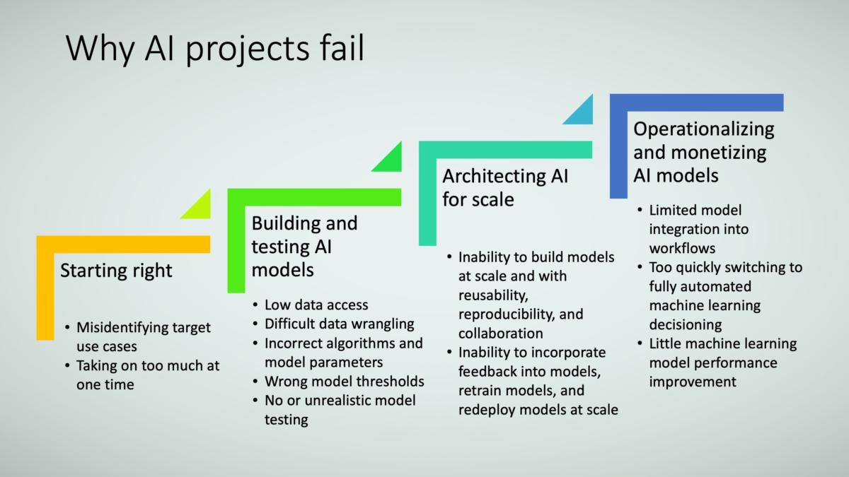
There are common ways that AI projects fail in the business environment, as Figure 26 shows. Any AI framework should address those pitfalls.

TRACE3

The first driver of failure is either selecting the wrong use case or taking on too many uses cases without sufficient capabilities and infrastructure. You can use the criteria described earlier to identify problems that better lend themselves to AI solutions. In addition, it is smart to set up a series of use cases that let capabilities and knowledge be built incrementally and with increasing technical sophistication.

Selecting the right use cases is best done collaboratively with:

• Line-of-business staff who know the business problems, contexts, and constraints, as well as the hypotheses they want tested.
• Business analysts who can ask questions that clarify the business intent and requirements, and who can identify the data sources and transformations.
• Data scientists who can formulate the machine learning and deep learning problem so that models can provide answers to the business’s hypotheses.
• Data engineers and IT resources who can provide access to the data.

Organizing and orchestrating these types of activities correctly upfront requires experienced cross-functional leaders who understand and can balance business impacts, operational drivers, workflow barriers and opportunities, data needs and constraints, and technology enablers.

The second driver is incorrectly building the AI models themselves. This consist of two elements:

• Even though data science, like other sciences, is experimental in nature (you don’t really know what the data will tell you until you work with it), the approach to data science should be well-defined, should be disciplined, and should speed time-to-value.
• Good data scientists can quickly experiment and iterate, learn from their experiments, distinguish between promising and ineffective approaches, and research and adapt cutting-edge methods if necessary. Good data scientists build MVPs (minimal viable products) in rapid, parallel fashion.

The third driver is lack of scale to quickly build and improve multiple AI models simultaneously. Frequently, this comes down to data scientists being able to work collaboratively, to reuse data pipelines, workflows, and models/algorithms, and to reproduce model results. Additionally, they need to be able to capture and quickly incorporate operational feedback (in the test, staging, or production environments) to further build scale. Accomplishing this requires both the correct infrastructure environment as well as a right-touch model governance approach.

The fourth driver of failure is an inability to operationalize and monetize AI models. Generally speaking, AI models are developed for one of two purposes:

• To find previously unidentified insights
• To automate decision making (for both cost reduction and efficiency/productivity).

Clearly, models that never make it out of the laboratory can’t accomplish these tasks.

Furthermore, not only do the models need to be deployed (that is, made accessible to people or systems), but they must be incorporated into workflows in such a way that they are “used” in operations, and exceptions (such as when models cannot make decisions with high probability of correctness) must be managed gracefully (such as through human intervention, model retraining, and model rollback). AI operationalization and monetization requires gradual but full model workflow integration, monitoring of data inputs and model performance parameters, and management of frequent model deployments.

How do I AI? An end-to-end AI solution framework

Finally, let’s tie all this together with an example AI solution framework shown in Figure 27.

TRACE3

There are four components:

• Data management.
• Model development.
• Model operationalization.
• Ensuring that the models are used, affect the business, and improve business metrics.

The first component, data management, is a normal part of current BI environments, so I don’t describe it here.

The second component, model development, consists to two broad areas:

• Defining and prioritizing use cases that are appropriate for machine learning models.
• Building the machine learning models at scale.

The third component, model operationalization, not only entails model deployment but also the process of continuous retraining and redeployment, model integration with operational workflows, and integration of operational feedback for model improvement.

The purpose of all of this is to monetize the models’ capabilities.

Finally, the fourth component, organization and business impact, is simple (and obvious) but vital to the future maturation of an organization’s AI capabilities. The function of this component is to ensure that the AI models are actually used by the lines of businesses (that is, they trust them and derive value from them) and that they are affecting business outcomes. Without line-of-business buy-in, the AI movement will rarely take flight.

Above these four components in Figure 27 are collaboration groups: IT, data engineers, data scientists, and lines of business. AI is a team sport.

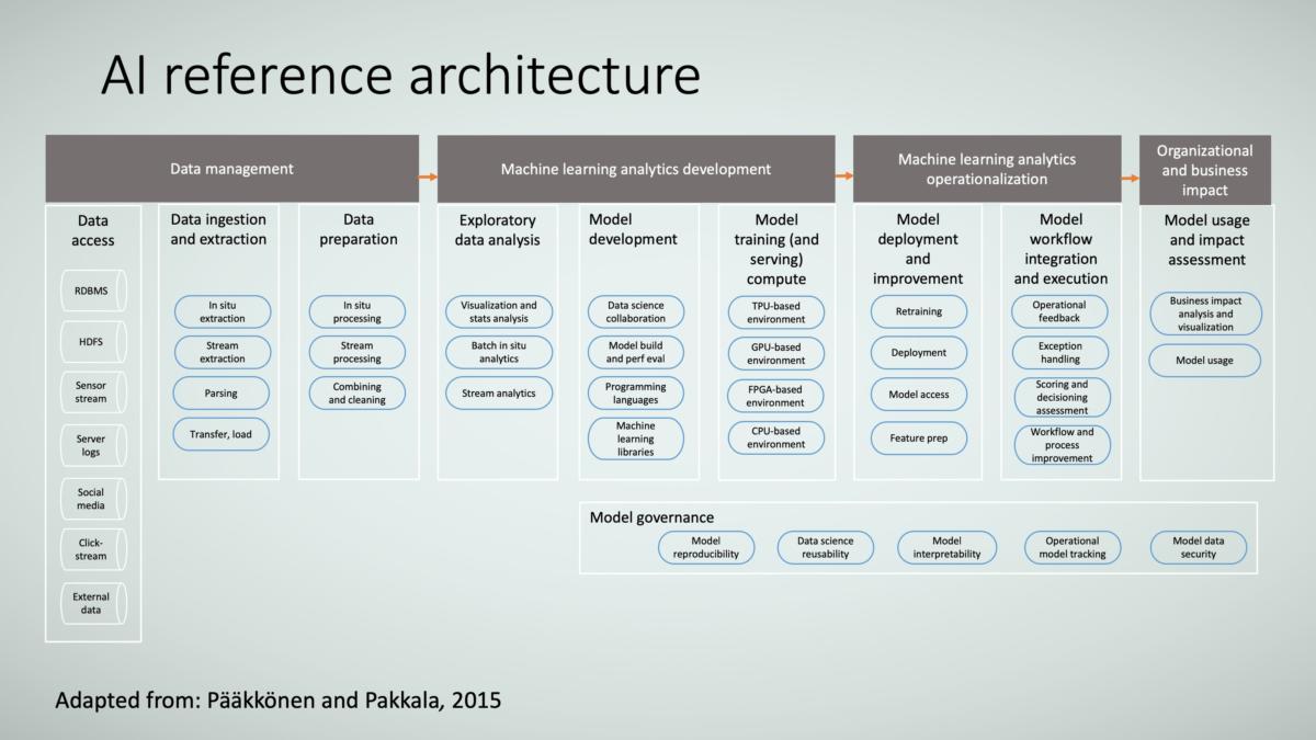
You can take these components and put a reference architecture around them (see Figure 28), adding a component called model governance to ensure that model reproducibility, data science reusability, and data scientists’ collaboration are achieved and to ensure that model retraining/rollback is possible when required.

TRACE3

Designing and implementing a solution like this reference architecture will support the AI solution framework with robustness, speed to market, and business outcomes.